Wave Tracker

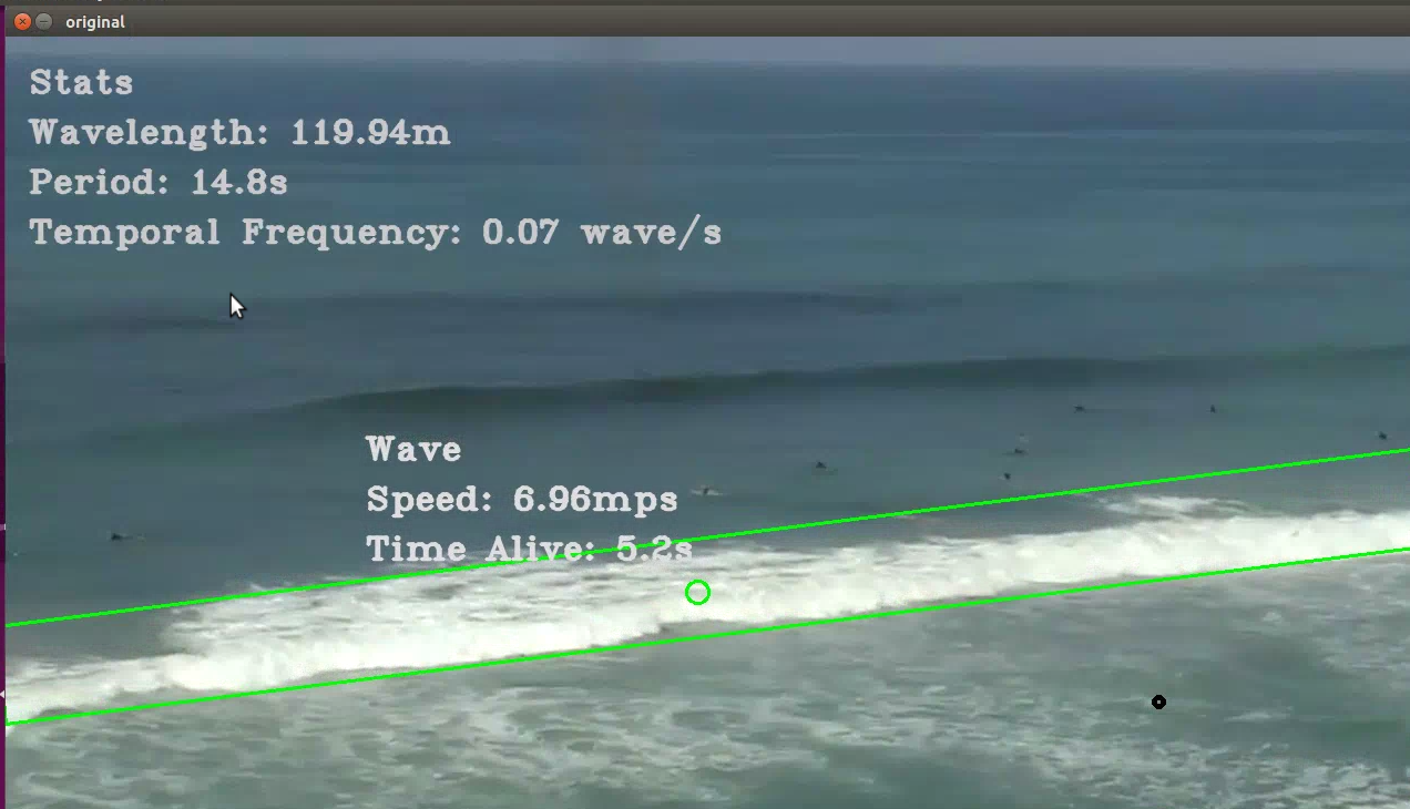
For an Advanced Computer Vision final project, my partner, Igor, and I extended a wave tracking library developed by GitHub user citrusvanilla. You can find our extension on GitHub here. Both the original project and our extensions use Python 2.7.16, NumPy 1.11.2, and OpenCv version 4.1.0.

Optical imaging has often been use to take measurements of ocean properties. With the development of new and more efficient methodologies as well as cheaper technology to perform them, it is now possible to perform an advanced analysis in real-time with inexpensive tools. This can help the already existing sensors used to measure the quality of the ocean at any given time for the beach-goers that would like to know such things.

To demonstrate this, we extend the previously implemented multiwavetracking Python Library. In particular, we added the following parameters to detect:

• Wavelength
• Period
• Speed
• Temporal Frequency

multiplewavetracking Library

Rather than redo what was already done in the GitHub project we decided to extend this approach for better results. We also decided to use a video clip from this project as the waves are most clearly demonstrated in it and it is perfect for the test purposes. The main idea described in this work is to use four general steps (preprocessing, detection, tracking and recognition) to recognize the wave objects on the video.

Preprocessing

In the preprocessing stage, the creator of the project resizes the image to a smaller scale to reduce further computational complexity. In order to focus on the waves, he uses the white of the foam created by the wave’s shoaling. To do this, a Mix-of-Gaussian background detecting mask is created and applied to the frame, removing the darker background to the waves and leaving a binary image. To remove remaining noise, a morphology operation is applied to the frame, removing non-salient foreground pixels that remained after the MOG step. This leaves only the larger patches that can be defined as waves with greater certainty.

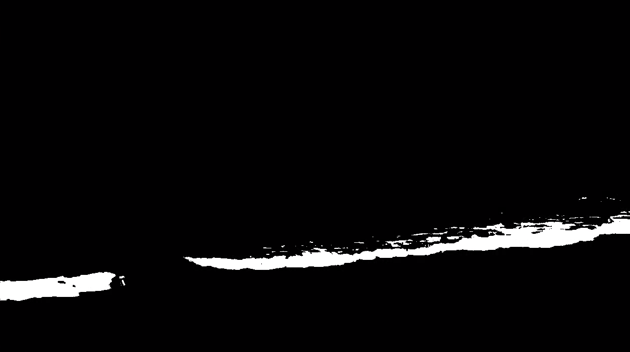
Rather than use the Mix-of-Gaussian, we used a binary thresholding function for less computational cost with similar results. It is resized after instead of before this step to ensure the foam doesn’t get interpolated out. The morphology step is kept for de-noising leaving a fairly accurate representation of the wave.

Detection

After the preprocessing, the contour detection method designed by Suzuki and Abe is used to make greater oblong shapes out of the remaining part of the waves, removing more false instances. They are also subjected to a threshold, removing those beneath a limit of area. We decided to keep this step the same, as it also involves creating an instance of the Section class for each remaining shape that holds all of our properties.

Tracking

The tracking step involves updating the wave objects created in the previous step based on the current frame. Because waves are generally going in one direction and are not expected to intersect and their shape follows a line orthogonal to their direction, this step is made simpler than would be without the assumptions. This step also allows for merging of wave objects that came from different contours, adding to the robustness of the algorithm.

Most of the tracking code remains the same in our implementation, following the same logic in updating the position and shape of the waves. On top of the functions called during this step, our own functions were added to calculate the slope and intercept parameters of the line describing the wave. This is used for the calculation of our added properties as described later.

Recognition

During this step, the waves are again tested to see if they are significant enough to keep by measuring the amount of pixels it occupies as well as its orthogonal displacement and checks if they exceed a predefined threshold. This eliminates false positives with cheaply calculated dynamics. This dynamics section remains the same in our implementation, and is also where our properties are calculated. The data collected during the tracking stage is compiled and displayed on the final screen.

Extensions

Here, I go into detail over how the different properties (velocity, wavelength, period) were calculated.

Velocity

To calculate the velocity, we measure the pixel distance that a wave moves from one frame to the next as shown in the below algorithm. This involves calculating a line function for the wave by calculating the slope of its points as well as the intercept. The slope is assumed to be the same in the next point, so the intercept is recalculated with the new centroid. An orthogonal line from the first point (the old centroid), using the negative reciprocal of the slope, is defined as well as the point at which it intersects with the second line (the current frame). The old centroid and this new point are used to calculate the Euclidean distance between the two lines.

Algorithm for calculating distance between two parallel lines

m_perp = -1 / slope

b_perp = y_p1 - x_p1 * m_perp

b_p2 = y_p2 - x_p2 * slope

Calculate point where perpendicular line intersects second line

x_inter = (b_p2 - b_perp) / (m_perp - slope)

y_inter = m_perp * x_inter + b_perp

Calculate distance between first point and the intersection point and multiply it by our pixel to meter ratio

return 1.25 * sqrt(y_p1 - y_inter)^{2} + (x_p1 - x_inter)^2)

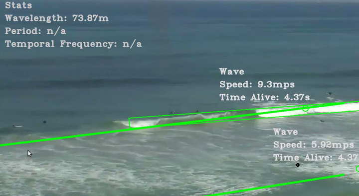
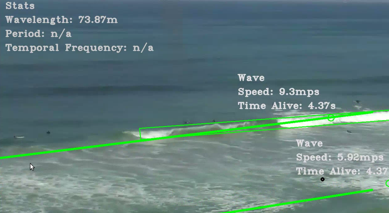
This distance is measured in pixels per frame, which does no good as a human readable measurement, so it is converted into meters per second. To convert the distance, it is multiplied by a hardcoded value representing the meters per pixel which we guess to bee 1.25 meters. To get the time unit right, it is then multiplied by the video's frame rate. This measurement is thresholded to prevent noise interfering with the value and then displayed by each individual wave.

Wavelength

The calculation of wavelength is done when at least two waves have entered the scene at the same time, and uses a similar method to that used in velocity calculation. The distance between parallel lines hitting the centroid of each waves with an averaged slope is calculated and displayed on the main text area. If there are more than two waves, the average of the wavelengths is taken, as waves often occur regularly and we wish for the most accurate representation of this value. When there is only one wave in the frame, the last calculated wavelength is kept on the screen until another wave appears.

Period

The period describes the amount of time it takes for a wave to travel its wavelength, or the time between the peak of one wave and the next passing the same point. The peak passing the point is what we did, arbitrarily selecting a point in the lower right-hand side of our video that we knew all waves would pass through. Each wave stores a boolean value that shows whether its passed the point yet to prevent recalculations after the fact. It is shown to have passed the point by passing the point through the slope-intercept function of the wave and seeing if the y value is greater than the one given by the equation. The frame that the wave’s line passes our point is appended to an array, and the difference between these points, once converted into seconds (again by multiplying with frame rate), is used as the period. Once there is more than two values in this array, the average difference is used for a more accurate measure of the period. The reciprocal of this value is calculated and represents the temporal frequency of the waves. Both of these values are displayed in the main statistics text in the top left corner of the screen.